Predicting the elusive origin of black holes in binaries
Published:
In the 20th century, black holes have transitioned from being but a mathematical curiosity pointed out by Karl Schwarzschild in the trenches of World War I to an observational feature that holds the potential to reshape our understanding of the Cosmos.
Thanks to the observations of light ejected from the vicinity of black holes, we now know that black holes constitute the endpoint of the life of very massive stars, that they harbour in the centre of most galaxies, that they act as an engine that fuels the rotation of galaxies, and that they make for an excellent background for the movie Interstellar.
Our understanding of how we got here, on Earth, a mere 14 billions years after the Big Bang, cannot be disentangled from our understanding of the birth and evolution of black holes.
Yet, we do not know why black holes are so abundant in the Universe.
Most of the black holes we have observed to date come in pairs, that is, binaries, and in the form of gravitational waves. There are two complementary philosophies as far as the formation of binary black holes goes. Some hypothesize that they form as a binary with one black hole and a star, which later on dies into a black hole amidst a flurry of ejected matter. Some hypothesize that black holes form dynamically (that is, purely gravitationally) in regions with overabundance of stars. Over the past few years, as gravitational waves were detected and became mainstream, astrophysicists have scrambled to provide predictions for the binaries’ abundance from either one of the two scenarios.
What has emerged is that a few candidates have all the markers of binaries formed dynamically. This is quite interesting, as these candidates can be used as laboratories for our understanding of dynamical interactions among black holes! What is particularly interesting is determining which dynamical formation path the black holes followed until their final configurations, and how many interactions they underwent. In turn, this will feed back into our understanding of the evolution of black holes, and our place in the Cosmos.
In this research, I train a machine-learning classification model to emulate a large suite of simulations from $\texttt{rapster}$, a dedicated software to simulate the abundance of black hole binaries formed dynamically. I then use this model in connection with messy data from dynamically-formed binaries to establish the formation path and how many interactions the black holes underwent en route to their final configuration.
Table of Content
Exploratory data analysis for a $\texttt{rapster}$ dataset
The $\texttt{rapster}$ code by Kritos et al. (2022) is a fast yet powerful code to simulate the dynamical formation of black hole binaries in globular clusters. Each run yields $O(10^6)$ binaries in the cluster starting from assumptions on the initial conditions of spins and masses of the black holes in the cluster. In this research I use datasets from 7 simulations.
Each dataset contains 28 features, ranging from the binaries’ masses and spins, the initial cluster mass, the amount of dark matter it contains and more (see the documentation for details). The datasets also retain information about the generation of black holes. A first generation (“1g”) black hole has not undergone any dynamical interactions before finding itself in a binary. A 2g black hole has undergone one iteration already, and so on. Moreover, the simulations retain information about the dynamical formation path of the black holes, i.e., if they were formed through exchange processes (“exc”), capture of one black hole by the other (“cap”), nonlinear interactions between three celestial bodies (“3bb”), from eccentricity resonances (the Zeipel-Kozai-Lidov effect, “ZKL”), and from derivatives of these resonances (“ZLK-v2”).
In what follows, I perform some basic steps for the exploratory data analysis (EDA) of a fiducial simulation from $\texttt{rapster}$.
To begin with, I sample $N=100000$ random data points from the simulations. This reduces the computational overhead from the million simulations I would need to carry over with the full dataset. By selecting the data points randomly, I make sure I am not over or underrepresenting corners of the parameter space. (I have double checked that the results below do not change with the full dataset.)
The first goal of this EDA is to define the target variables. We have two questions in mind: A) “which generations do the observed black holes pertain to?” B) “what formation channels do they come from?”
We use $\texttt{pandas}$ to wrangle the two columns with the generations of the individual black holes and create a column with our target variable for question A). We define
\[y_{\text{gen}}=[\text{"1g+1g"}, \text{"1g+2g"}, \text{"2g+2g"}],\]as the (target) set of binary configurations in which we have two, one or no first-generation black hole respectively. We mask generations higher than the second as they constitute outliers in our datasets.
We then define the formation path column as the target variable for question B),
\[y_{\text{form}}=[\text{"exc"},\text{"cap"}, \text{"3bb"}, \text{"ZLK"}, \text{"ZLK-v2"}].\]The second goal of the EDA is to establish the predictors. For this, I perform a correlation study among $y_{\text{gen}}$, $y_{\text{form}}$ and the remaining 26 variables. I find that the parameters that mostly correlate with the target variables are the masses $m_{1,2}$ and spins $\chi_{1,2}$ of the two black holes, with Pearson correlation coefficients $0.33 < \sigma_{X_1X_2} < 0.95$.
For the formation channels, the initial cluster mass and redshift ($M_{\text{cl}}$, $z_{\text{cl}}$) to also be somewhat (anti-)correlated with $y_{\text{form}}$ (with $ -0.33 <\sigma_{X_1X_2} < 0.05$). I also find the log (base 10) of the total mass $\log M_{\text tot} = \log (m_1+m_2)$ and the mass ratio $q = m_1/m_2$ to give more stable fits.
All in all, I set the predictors to
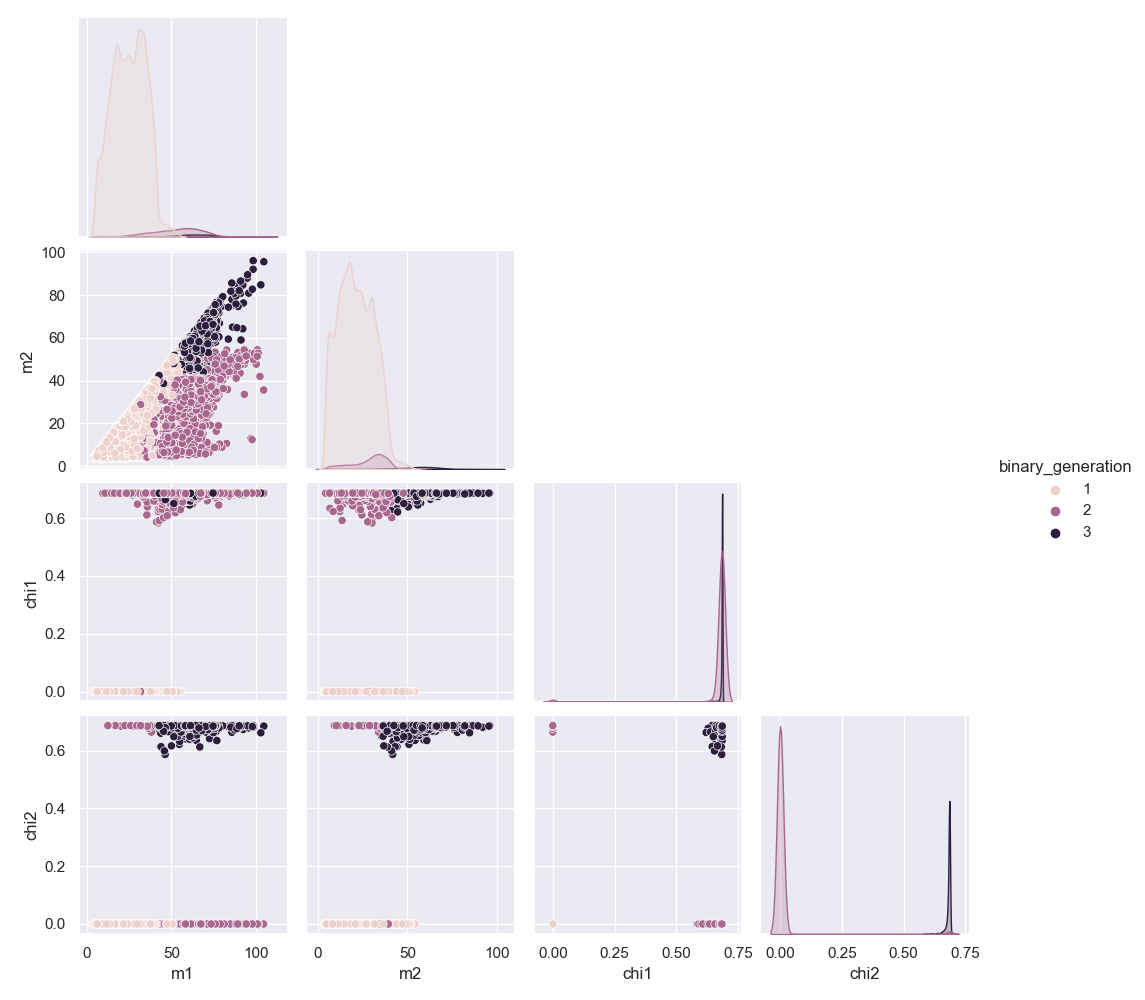
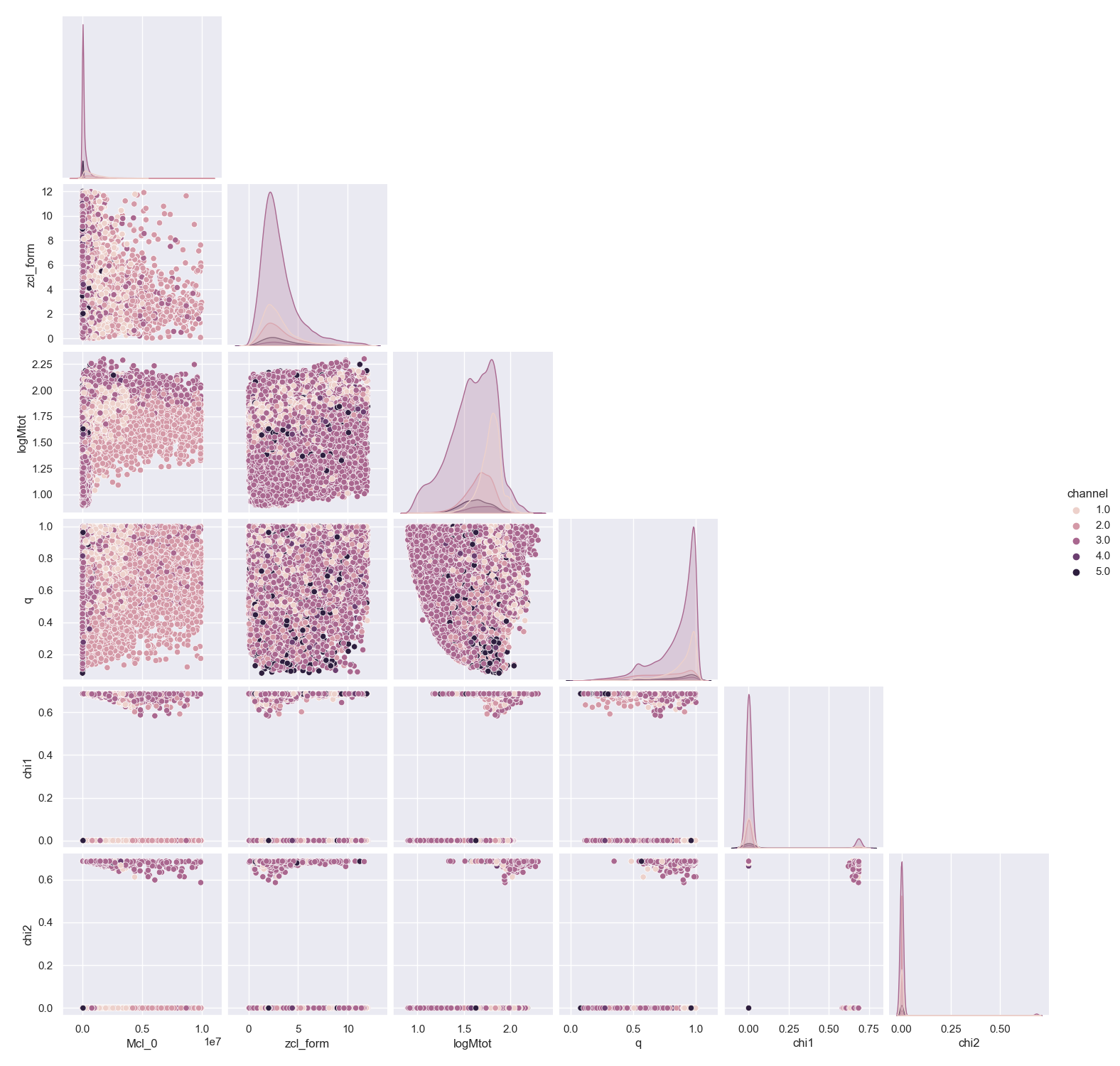
\[X_{\text{gen}}=[m_1,m_2,\chi_1,\chi_2],\] \[X_{\text{form}}=[\log M_{\text tot}, q,\chi_1,\chi_2, M_{\text{cl}}, z_{\text{cl}}].\]The third and final goal of the EDA is to visualize the set of predictors and their relation with the target variables. I do so hue-ing the latter in a corner plot of the former using $\texttt{seaborn}$ (notice that the labels refer to the index of the predictors’ sets). The spins help break the degeneracy between the generations of black holes: because of this, I expect the fits for this target variable to perform well. The same unfortunately cannot be said for the formation channels, which exhibit no discernible patterns.
Training and validation of the model
Following the data preparation steps outlined above, I split the dataset into training (70%) and test (30%) datasets using the $\texttt{train_test_split}$ function from $\texttt{scikit-learn}$. Then, I explore various classification algorithms and inspect their $R^2$ scores.
Starting from fits for $y_{\text{gen}}$, I find:
- Gaussian Naive Bayes, $R^2=0.99$.
- Multinomial Naive Bayes, $R^2=0.99$.
- SVM, $R^2=0.94$.
- K-means clustering, $R^2=0.40$.
- Logistic Regression, $R^2=0.99$.
- Decision Tree Classifiers, $R^2=0.99$.
- Random Forest Classifier, $R^2=1.00$.
- XGBoost, $R^2=1.00$.
Aside from K-means clustering, all the models perform really well, as expected from the inclusion of spins in the dataset. Given the wealth of algorithms to choose from, I opt for decision-tree based algorithms due to their interpretability. A simple decision tree algorithm performs really well already with an $R^2=0.99$: in raw numbers, it predicts 28272 “1g+1g”, 1424 “1g+2g” and 295 “2g+2g” binaries. The test set has 28252, 1444 and 295. Pretty accurate!
However, decision trees suffer from biases in the selection of the root node. By switching to a Random Forest (RF) algorithm, the bootstrapping of the dataset inherent to this method allows to improve the model even further. I have checked that the RF correctly predicts all “1g+1g”, “1g+2g” and “2g+2g” configurations, also when resampling the original simulations dataset or using it in its entirety. For this reason, I choose a RF algorithm to predict the black-hole generations.
Below is an example of the 1444 correctly predicted “1g+2g” binaries in the $m_1 - m_2$ plane, which I have chosen as the header of this post.

When it comes to predicting $y_{\text{form}}$, I find models to yield lower but still reliable $R^2$. For the same reasons as above, I pick a RF classification algorithm that yields $R^2=0.78$. The confusion matrix for the predicted values can be used to inspect the false positives/negatives. It looks as follows.
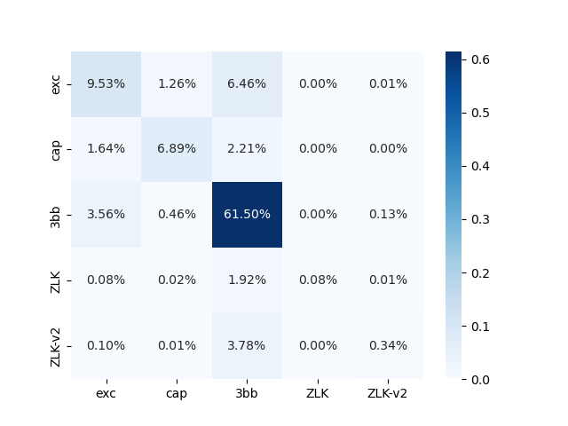
As the diagonal terms tend to dominate percentages with same rows/columns, we know there are no cases in which a formation path is preferentially biased towards an incorrect value. Because of this, and noting that the approach could be improved even further by reweighing the off-diagonal terms for more stable fits, I proceed to apply the models to interferometers’ data.
Applying the models to interferometers’ data
The first problem to tackle to apply the models to data is conceptual: the classification algorithms take point estimates for the masses and spins without taking errors into account. Moreover, they are inherently frequentist and work best for populations of black holes in which we can neglect individual errors.
The data from gravitational-wave interferometers does not unambiguously give us populations of dynamically-formed black holes. It does give hints, however, that certain individual events are more likely to be formed dynamically. These are black holes that have masses higher than what predicted from other formation scenarios, or spins that do not vanish. One such example is GW190521, a black-hole binary in which the individual masses are too big to be explained by any scenario other than dynamical interactions.
When data reaches us from interferometers, it has already undergone a Bayesian treatment. That is, the data we get has masses and spins repoted as credible intervals. For example, the masses of GW190521 are reported as below. (I have used $\texttt{PESummary}$ to reproduce the plot).
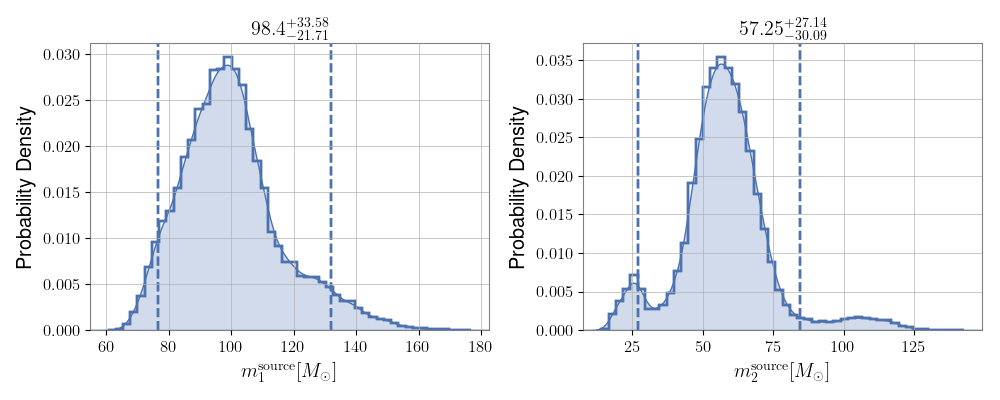
The credible intervals are a result of Monte Carlo analyses, and they are not trivially incorporated in the classification models above. However, it suffices to realize that Monte Carlo analyses involve successive steps in which the true posterior is sought after. At each iteration, a set of the masses, spins and other parameters of the binary is recorded. More concretely, one can visualize the posteriors above in slices of the parameter space. For the $m_1-m_2$ plane used in the header of the post, the final Monte Carlo analysis looks like the following:
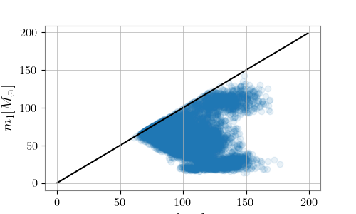
Contour plots (and thus 1-D marginalized posteriors) are drawn from concentrations of the “points” accumulated with successive iterations.
The key realization in my work is that successive iterations in Monte Carlo analysis of individual gravitational-wave events can be treated as independent predictors for the machine-learning classification algorithms. I use each quartet of masses and spins measured by interferometers as input for Equations (2) and (3) above [making random choices for $M_{\text cl}$ and $z_{\text cl}$ in (3)], and repeat the procedure for the $N$ samples from the Monte Carlo analysis. Finally, I average over the $N$ predictions for generation and formation path of the black holes and report a single, averaged p-value.
Using the fiducial simulation from $\texttt{rapster}$, for instance, I find that GW190521 has a 21% chance of having gone through no dynamical interactions, a 53% chance that one of the two black holes in the binary underwent at least one interaction, and a 26% chance both did. Moreover, I find no evidence that exchange processes or eccentricity resonances have formed the binary, and an equal chance that three body interactions or two-body captures did.
While it is too early to claim any astrophysics from the statement above, the illustration above is a good starting point for future research. I plan to extend the simulation datasets to include evermore astrophysics, apply the models to different families of black holes (from those as massive as the Sun to those as massive as the Milky Way), and explore how the answers above change when we consider different initial assumptions for the $\texttt{rapster}$ datasets.
In the meantime, the illustration above serves as an example of how we can use machine learning to find out the origin of black holes.
The analysis discussed above can be reproduced with codes at this link.
