An A/B test for biased gravitational-wave signals
Published:
One of the most astonishing features of gravitational-wave (GW) data analysis studies is that we can reconstruct the evolutionary history of the black holes or neutron stars that generate them.
By now, large collaborations routinely inspect signals in search of the parameters that best describe these sources. The most sought after parameters are the masses and the spins (metrics of rotation) of the celestial objects, which maintain traces of their distribution in the Universe and thus evolution.
The parameter estimation procedure is conceptually simple. A data stream
\[d(t) = n + h(t,\theta),\]containing detector noise $n$ and a potential signal $h(t,\theta)$ described by parameters $\theta$, is fed into a probability likelihood that is optimized to look for the most likely parameters. The procedure requires a very accurate understanding of what the shape of the signal is, and it relies heavily on the assumption that no other signal is present in the data.
While this is a good assumption for current parameter estimation studies, what will happen when next-generation detectors will detect thousands upon thousands of GW events?
In this case, the data stream looks more like
\[d(t) = n + h(t,\theta) + \Delta H_{\text{conf}},\]where $\Delta H_{\text{conf}}$ describes all the unmodelled signals in the data and acts like an additional source of noise. Could this “confusion” noise be problematic for the estimation of $\theta$?
Despite the formulation above, the question can be recast as an A/B test, in which A represents the hypothesis that the parameter estimation of $h(t,\theta)$ will not be affected, or biased, by the presence of the underlying unmodelled signals, and B represents the hypothesis that it will.
In this research, I have co-developed an A/B hypothesis testing formalism to inspect whether signals detected with future detectors will be affected (“biased”) by the presence of thousands of unmodelled signals in the data.
Table of Content
Defining the A/B test
Parameter estimation studies of GW events are usually performed within a Bayesian formalism, in which parameters $\theta$ are reported as posteriors within a credible interval. Due to the uncertain nature of statistics, we do not have access to the parameters that describe the source exactly. However, if noise is kept under control, we can say that the observed parameters lie within a credibility region of 68% significance (or $1\sigma$) around the true parameters.
Whenever the posteriors are well described by a Gaussian – for instance when the sources are loud, – the error at the 1$\sigma$ confidence can be approximated by the Fisher matrix. (Not to be confused with the Fisher exact metric.) The steps leading to the derivation of the Fisher matrix in a GW context can be found in equations (1) to (9) of the method’s paper. What is interesting to point out here is that the Fisher matrix $\Gamma_{ij}$ is a (semi)-analytical formula to cheaply and reliably estimate the variance at the 1$\sigma$ level. In math parlance, it is defined as
\[\Gamma_{ij} = \left(\frac{\partial h}{\partial \theta^i},\frac{\partial h}{\partial \theta^j}\right),\]where $(\cdot, \cdot)$ can loosely be thought as the “least square” distance between the signals.
It can be demonstrated that errors from the Fisher matrix capture the spread around which we expect shifts in the parameters to lie due to random noise fluctuations. The formula that describes this is
\[\Delta\theta^{i} = \sqrt{(\Gamma^{ij})^{-1}}.\]In other words, the Fisher matrix gives access to the error around the true, inaccessible parameters of the source. The observed median moves around the true parameters as a result of the effect of detector noise, but roughly around the 1$\sigma$ values.
Let’s now introduce more signals in the data. While the formalism below generalizes to a variety of situations in which modelled, unmodelled signals or a combination of both are added to the data, it can be easily illustrated with a simpler example in which we have only one overlapping signal. That is, in this case $\Delta H_{\text{conf}} $ is composed of another signal, as shown below.

If the overlapping signal is ignored in the parameter estimation of the reference signal $h(t,\theta)$ in Eq.(1), there may be trouble. The increase in the size of the effective noise, composed of both detector and confusion noise, may push the observed median for the parameters $\theta$ further than the $1\sigma$ level described by the Fisher matrix. In this occurrence, the parameter estimation is said to be biased.
Understanding and dealing with multiple signals in the data is of paramount importance for the science case of near-future multibillion-dollar gravitational-wave experiments, but biased parameter estimation studies may lead us to infer the wrong science from black holes and neutron stars. In section 3 of the paper, I generalized a previous approach by (Cutler & Vallisneri, 2007) to calculate the parameter shift $\Delta \theta$ due to the presence of confusion noise from overlapping signals. The formula reads
\[\Delta\theta_{\text{conf}}^i = (\Gamma^{ij})^{-1}\left(\frac{\partial h}{\partial \theta^i},\Delta H_{\text{conf}} \right).\]The A/B test is performed comparing equations (4) and (5). If $\Delta\theta_{\text{conf}}^i$ is larger than $\Delta\theta^{i},$ the shift in the parameters due to the overlapping signal will favour hypothesis B in which the parameter estimation is biased. If $\Delta\theta^{i}$ is smaller, the parameter estimation is not biased and hypothesis A is favoured.
Validating the model
I validated the model extensively in the paper, where I introduce mock data for the future spaceborn gravitational-wave detector LISA and for next-generation ground-based detectors such as the Einstein Telescope and Cosmic Explorer. As standard in the field, I validate the Fisher-matrix based estimates above using Markov Chain Monte Carlo (MCMC) simulations. I explored a variety of situations, in which both unmodelled signals and modelled signals that were inaccurately removed were present in the data. Here is the repo with all the examples I came up with. In all cases, I find equation (3) to accurately predict the size and direction of the bias for all the parameters involved.
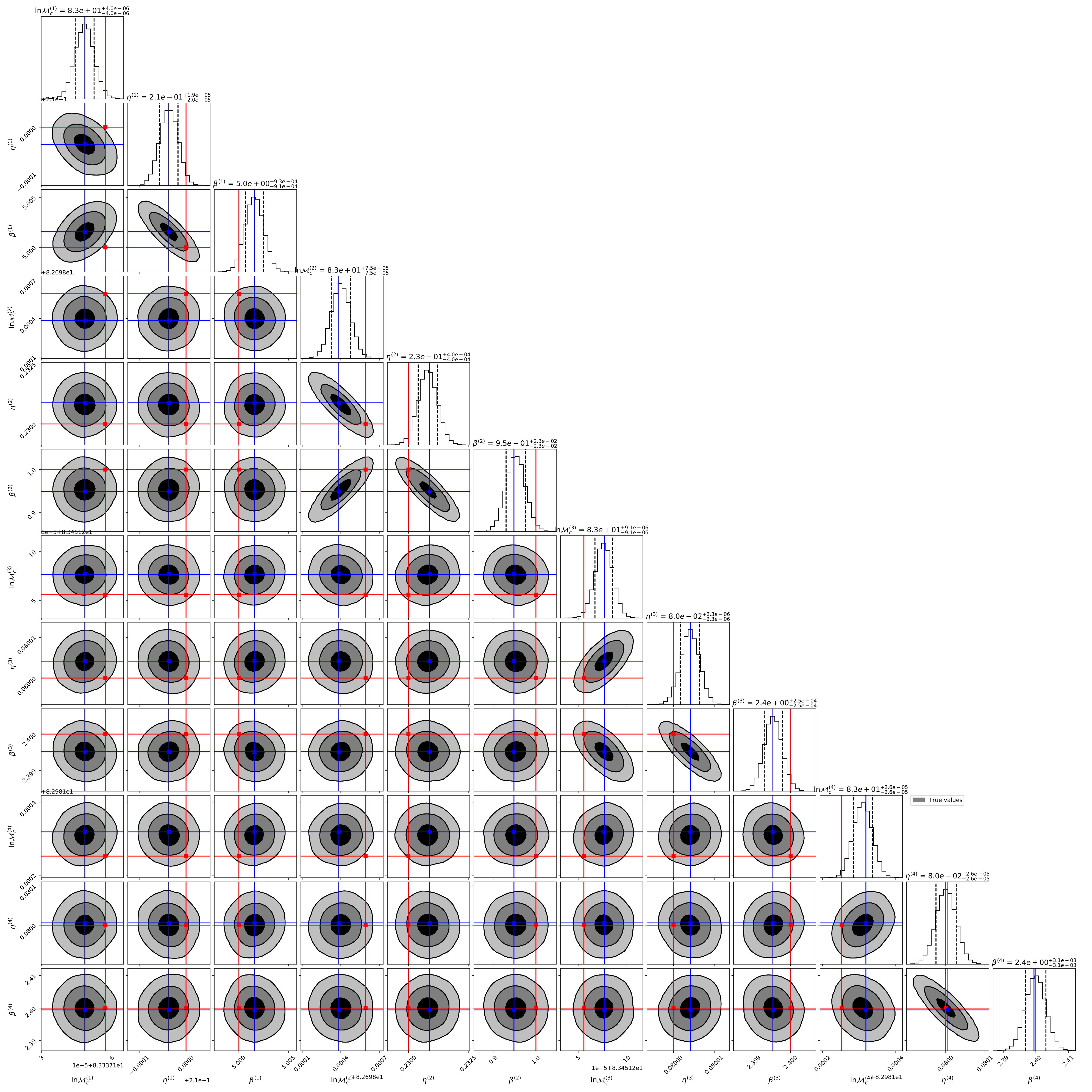
Below is an example of the recovery of the biases on the parameters of 4 incorrectly-modelled signals in the LISA detector, and in the presence of unmodelled noise.

I show in red where the true parameters lie. As expected they lie beyond the 1$\sigma$ contours that would be described by the Fisher matrix, confirming that confusion noise leads to biases in the parameter estimation of $h(t,\theta)$. In blue, I show the predictions obtained with our formalism.
Despite the complexity of the parameter space, the formalism can predict exactly where the biased parameters lie. Neat!
The formalism can be very useful to forecast when and where in the parameter space the posteriors of GW events will be biased. As briefly touched upon above, this is especially in the science case of near-future detectors. In fact, in (Reali, Antonelli, et al., 2022) we describe how the formalism could be used in a more astrophysically realistic context, and in particular for next-generation ground-based detectors.
